
model download link: https://www.blendswap.com/blend/23392
What is ray/path tracing anyways?
Ray tracing is a way for the computer to realistically simulate light’s behavior in real life that could yield photorealistic images if everything is done right. A ray tracing algorithm simulates light by shooting rays from each individual pixel set by the camera canvas defined by the user. The amount of rays shot out will be determined by the resolution of the camera, and each individual ray is calculated to see if it intersects the geometry of the mesh. When the ray hits the object, some percentage of it is absorbed and some are reflected, in some cases with transparent or semi-transparent materials the rays could also transmit through the object (aka shoot through the object). The amount of rays absorbed is determined by the color of the material defined on that specific geometry, and similarly that goes for the amount of rays reflected. The amount of rays transmitted through the material is determined by the transparency of the material. Ray tracing can also achieve refraction–that is the bending of light– through an object, which is governed by the IOR (index of refraction) of the object set in the materials panel, which in turn can achieve caustic effects (say you shine a strong light through a bottle of wine, it casts a bright spot of light that’s slightly paler than the wine itself but on the table it sits on. But this is only able to be achieved through path tracing since only that can achieve multiple light bounces required for caustics).
When the rays are shot from the camera, it follows the principles of physics in real life, such that the amount of rays shot will be equal to the amount of rays reflected and absorbed. It also follows the law of reflection, that is the angle of the incident ray is identical to that of the reflected ray. As the ray hits the surface, multiple other rays are created, such as diffuse rays, reflection rays, and transmission rays (through transparent or semi-transparent materials), which would also be calculated until some rays hit the light source and the data is recorded on that individual pixel, which is called a sample. Initially, the image will be noisy, since there aren’t many rays that actually hit the light source, and there would be a lot of dark spots on the image, creating noise. As sample counts increases, more and more rays starts hitting the light source, evening out the original noises. The noise can be further decreased using a denoiser, which can speed up the renders significantly since the computer would use a lot less samples than without a denoiser to achieve similar image quality.

Source: https://www.scratchapixel.com/images/upload/introduction-to-ray-tracing/reflectionrefraction.gif

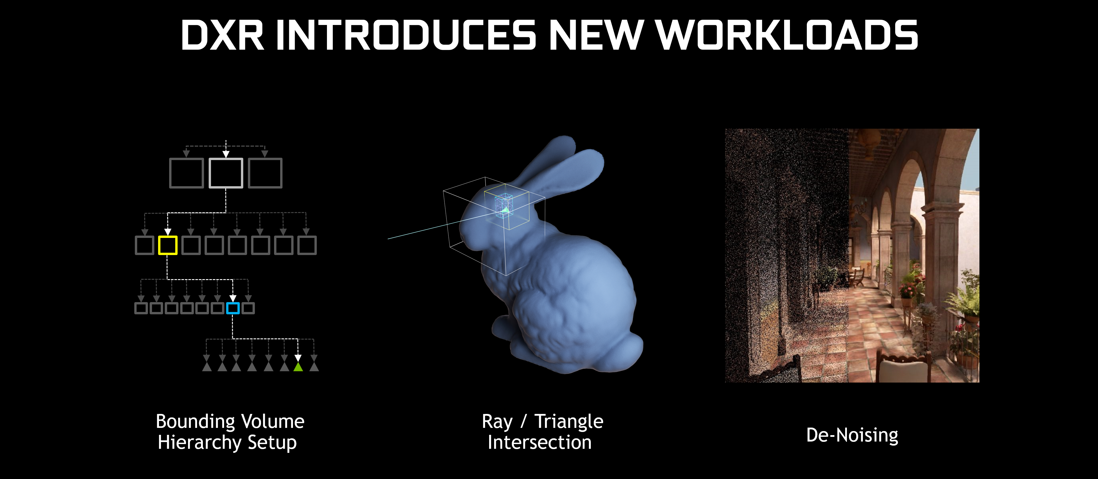
Source: https://images.nvidia.com/content/images/geforce-gtx-dxr-ray-tracing-available-now/geforce-rtx-gtx-dxr-introduces-new-workloads.png
The performance of ray tracing
The ray tracing algorithm is actually very efficient for the kind of complexity it is simulating. Ray tracing is essentially a glorified version of the Monte-Carlo Tree Search; it is very easily parallelized, both across CPU cores and the many GPU cores, even across multiple chips as it is almost as if each pixel is individually simulated. That means in order to scale up ray tracing performance, you just need more cores in a computer and more powerful cores, and it scales almost linearly with the amount of cores your computer has. However, even with modern computers hitting near 20TFLOPs on a single GPU, ray tracing is still an incredibly demanding task since it has to physically trace billions and billions of rays with the most intensive calculation being whether the ray intersects some part of the geometry or not. This is the reason why so much efforts are invested into accelerating ray tracing, both from a hardware and software level. The most prominent accelerating method is BVH structure, which essentially computes a bounding box around the objects that will be ray traced, and limit the rays from the camera to only trace when it is within the bounding box. The second most common method is to use a denoiser, which smooths out the noises and cleans up the images to look better.
If denoising is so good, why not use it on every single render then?
Denoising has several drawbacks. First of all, it’s not realistically simulating all the lights anymore, but instead it is trying to interpolate what is going on between the pixels and “faking” the image in the process of doing so, which have nothing to do with tracing light rays. Secondly, since denoising interpolates pixels, when rendering an animation, every single frame is very slightly different in some cases, and vastly different in other cases. In every single frame the denoiser would introduce some randomness of noise, since the values of the surrounding pixels around the noise pixels would change, which would make the animation look unpleasant to the human eye and it seems like there’s a very heavy film grain effect applied to it. Finally and most importantly, as denoiser interpolates the relationship between pixels surrounding the noises, it average out the minute details that might be present in a render such as a texture, making it seem blurry, unrealistic, and much lower resolution than what it actually is before denoising.


This GIF demonstrates a comparison of image quality and sample rate without denoising applied, and also compares the different amount of time it takes to render on a Ryzen 7 1700 system at 3.85GHz, DDR4 3000 Dual Channel RAM, and an Nvidia Titan V running at 1800MHz core and 1040MHz HBM2 during actual load. (Contains some noise introduced by GIF compression)
There is a significant trade-off between render time and quality. The ground truth image, which is render at 20000 samples, took over 15 minutes to complete on a relatively low resolution of 960×540 pixels. The difference between the low samples are huge. However, as you approach higher and higher samples, the differences becomes less and less apparant. Even at 20000 samples, there are still a tiny amount of noise despite the insanely long render time, showing a significant diminishing return. This kind of noise can be easily smoothed out with either traditional and AI denoisers without losing much image fidelity.


1 Sample, Blender Denoiser 
2 Samples, Blender Denoiser 
4 Samples, Blender Denoiser 
8 Samples, Blender Denoiser 
16 Samples, Blender Denoiser 
32 Samples, Blender Denoiser 
64 Samples, Blender Denoiser 
128 Samples, Blender Denoiser 
256 Samples, Blender Denoiser 
512 Samples, Blender Denoiser 
Ground Truth (20000 Samples)
This GIF demonstrates a comparison of image quality and sample rate using the traditional Blender denoiser, and also compares the different amount of time it takes to render on a Ryzen 7 1700 system at 3.85GHz, DDR4 3000 Dual Channel RAM, and an Nvidia Titan V running at 1800MHz core and 1040MHz HBM2. (Contains some noise introduced by GIF compression)
You might be able to notice that the low sample “denoised” images look extremely terrible, especially with the ones with only 1 and 2 samples, as you can barely interpret the image as a Lamborghini supercar at those sample counts. In my opinion, the low samples “denoised” images look even worse than the ones without denoise since at least your eyes can perceive it as a Lamborghini rather than not knowing what it is. At the same time, there is also a significant increase in render time when using low sample rates. Despite the GIF making it seem that at above 256 samples there are a lot of noise, in reality there is almost zero noise whatsoever and that was due to the GIF compression algorithm. Overall, the Blender denoiser works relatively well at a moderate amount of samples as the difference is very minute between 256 samples denoised and 20000 samples ground truth. The only difference is that as previously mentioned, a denoiser would smooth out the sharp edges a bit and also smooth out the texture, making them less apparant. It also has relatively little overhead at only around 0.8s extra per render.


1 Sample, OptiX AI Denoiser 
2 Samples, OptiX AI Denoiser 
4 Samples, OptiX AI Denoiser 
8 Samples, OptiX AI Denoiser 
16 Samples, OptiX AI Denoiser 
32 Samples, OptiX AI Denoiser 
64 Samples, OptiX AI Denoiser 
128 Samples, OptiX AI Denoiser 
256 Samples, OptiX AI Denoiser 
512 Samples, OptiX AI Denoiser 
Ground Truth (20000 Samples)
This GIF demonstrates a comparison of image quality and sample rate using the D-Noise AI denoiser, and also compares the different amount of time it takes to render on a Ryzen 7 1700 system at 3.85GHz, DDR4 3000 Dual Channel RAM, and an Nvidia Titan V running at 1800MHz core and 1040MHz HBM2. (Contains some noise introduced by GIF compression)
The AI denoiser does a significantly better job at lower sample counts compared to the traditional Blender denoiser. However, it makes the geometry significantly deformed, which unlike the traditional denoiser only with the edges significantly thickened but retained the general shape, though at the same time it did almost smooth out all the noises in the image. The denoiser has a slightly higher overhead compared to the traditional Blender denoiser at around 1.8-2s range. The advantage of this denoiser is that you don’t really lose the sharp edges of the geometry, especially when at mid-high sample count such as 256 and 512 samples, there’s virtually no difference between the ground truth and the denoised images. Although the denoiser is still not perfect, as it distorts the geometry of the object at lower sample rates, and even at 128 samples which is where the traditional denoiser did a significantly better job in my opinion as it both retained the geometry of the car as well as smoothed out the noise. Both denoisers lost some details in the reflection where there is supposed to be bright white stripes, but at higher sample counts it is not as apparant, and both denoisers are significantly faster than rendering the image at 20000 samples with a close enough result.

You must be logged in to post a comment.